Unveiling cinematic insights: analyzing my Letterboxd data

Introduction
Letterboxd is a fantastic platform for film enthusiasts to track and share their movie-watching experiences. Apart from being a hub for movie reviews and social interaction, it also provides a valuable dataset that can be harnessed to gain insightful statistics about your film preferences and habits. In this blog post, I will guide you through the process of extracting and analyzing your Letterboxd data, enabling you to uncover intriguing patterns and trends hidden within your cinematic journey.
Step 1: Exporting Your Letterboxd Data
To get started, you need to export your Letterboxd data. Follow these steps:
- Log in to your Letterboxd account.
- Click on your profile picture and select “Settings.”
- Scroll down to the “Data Export” section.
- Click on the “Request Data Export” button.
- Wait for an email notification confirming that your data is ready for download.
Once you receive the email, download the data export file. It will likely be in a compressed format, such as ZIP. Unzip the file to access the data in a CSV format.
To get started, we load our data from two CSV files: watched.csv containing details about the movies we’ve watched and ratings.csv containing our ratings for those movies. We then merge these datasets on common columns: 'Date', 'Name', 'Year', and 'Letterboxd URI'.
import pandas as pd

WATCHED_DATA_FILE = "/path/to/watched.csv"
RATING_DATA_FILE = "/path/to/ratings.csv"

watched_data = pd.read_csv(WATCHED_DATA_FILE)
rating_data = pd.read_csv(RATING_DATA_FILE)

watched_movies = watched_data.merge(
    rating_data, on=["Date", "Name", "Year", "Letterboxd URI"], how="left"
)
Step 2: Enriching Genre, Director, and Runtime Information
We complement our dataset by fetching genre, director, and runtime information from the TMDb API (I relied on the tmdbsimple wrapper) using the fetch_movie_details function.
Replace YOUR_API_KEY with your actual TMDb API key, which you can obtain by signing up for a free TMDb account and generating an API key.
import tmdbsimple as tmdb

def fetch_movie_details(movie_name):
    try:
        search = tmdb.Search()
        response = search.movie(query=movie_name)
        if search.results:
            movie_id = search.results[0]["id"]
            movie = tmdb.Movies(movie_id)
            details = {
                "Genre": [genre["name"] for genre in movie.info()["genres"]],
                "Director": ", ".join(
                    [
                        crew["name"]
                        for crew in movie.credits()["crew"]
                        if crew["job"] == "Director"
                    ]
                ),
                "Runtime": movie.info()["runtime"],
                # Add more details as needed
            }
            return details
        else:
            print(f"Movie with name '{movie_name}' not found.")
            return {}
    except Exception as e:
        print(f"Error occurred while fetching details for movie '{movie_name}': {e}")
        return {}

tmdb.api = 'YOUR_API_KEY' # Set your TMDb API key here
watched_movies['Movie Name'] = watched_movies['Name'].str.strip()  # Remove leading/trailing whitespace
movie_details = watched_movies['Movie Name'].apply(fetch_movie_details)

# Update the respective columns in the watched_movies DataFrame
watched_movies['Genre'] = movie_details.apply(lambda x: x.get('Genre', None))
watched_movies['Director'] = movie_details.apply(lambda x: x.get('Director', None))
watched_movies['Runtime'] = movie_details.apply(lambda x: x.get('Runtime', None))
Step 3: Key Analyses
Let’s now perform an Exploratory Data Analysis (EDA) to gain insights on your watching habits.
During my journey, I discover that I logged 391 watched movies, of which I rated 118 and my average rating is 3.40.
Month seasonality
Let’s visualize the distribution of movies watched over time.
# Count the number of movies watched per month
movies_watched_by_month = watched_movies.groupby(watched_movies["Date"].dt.to_period("M"))[
    "Name"
].count()

# Plotting a bar chart of number of movies watched per month
plt.figure(figsize=(12, 6))
sns.barplot(
    x=movies_watched_by_month.index, y=movies_watched_by_month.values, palette="muted"
)
plt.xlabel("Month")
plt.ylabel("Number of Movies Watched")
plt.title("Number of Movies Watched Over Time")
plt.xticks(rotation=45, ha="right")
plt.tight_layout()
plt.show()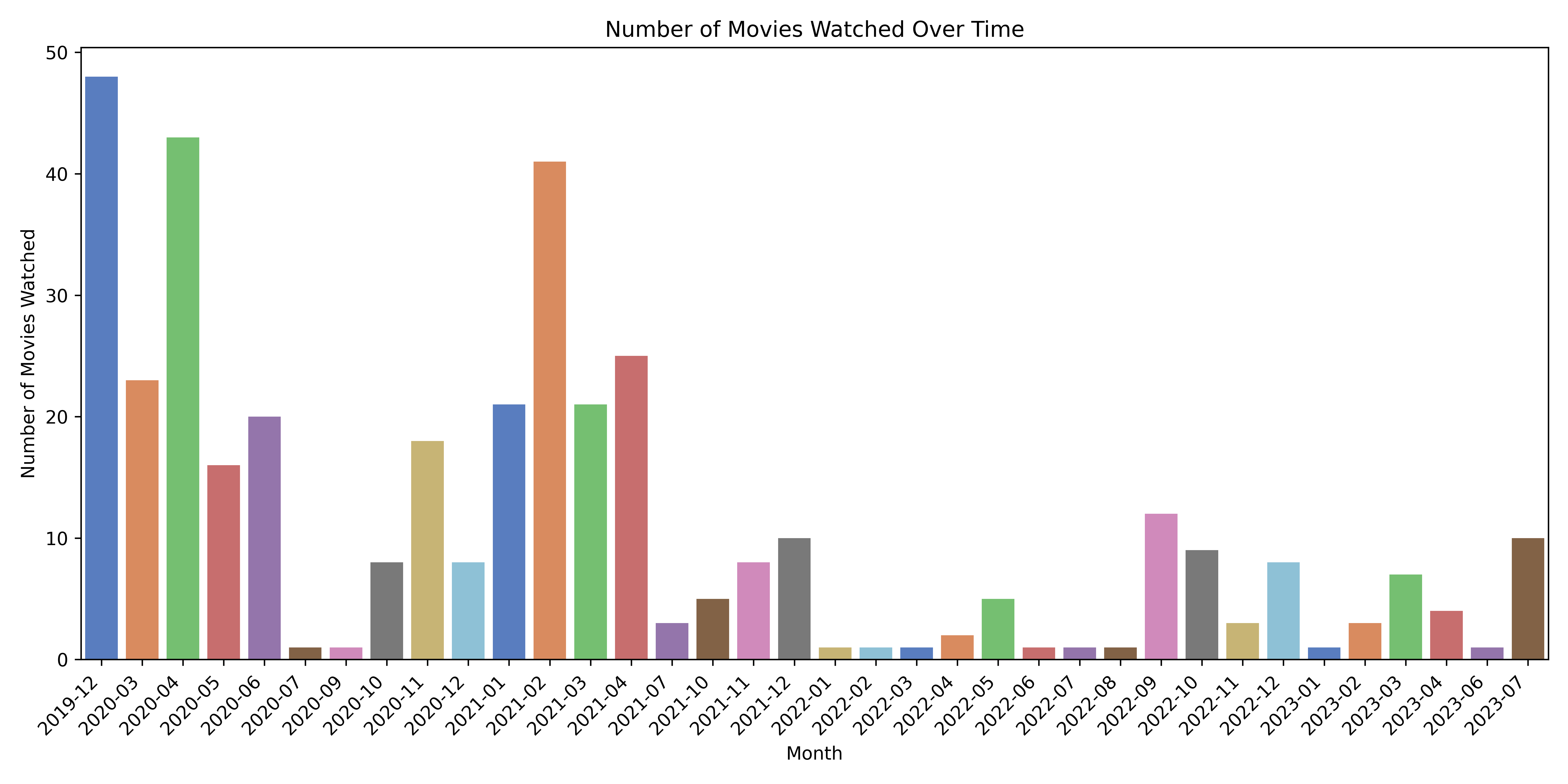
It came as no surprise that during covid lockdowns in 2020 and 2021 I watched a looooot of movies. This July 2023 is different from the others as I managed to go everyday to the Dolce Vita sur Seine open air cinema festival and was able to watch a lot of stuff. Moreover, the weather in Paris this summer is awful, so late sunsets at Paris Plage are replaced with the vision of movies. Last but not least, it is Barbie month!
Day of week seasonality
Let’s visualize the seasonality of movies watched over time.
watched_movies["Date"] = pd.to_datetime(watched_movies["Date"])
watched_movies['Day of Week'] = watched_movies['Date'].dt.day_name()

# Count the number of movies watched on each day of the week
movies_watched_by_day = watched_movies['Day of Week'].value_counts()

# Sort the days of the week in the correct order
days_order = ['Monday', 'Tuesday', 'Wednesday', 'Thursday', 'Friday', 'Saturday', 'Sunday']
movies_watched_by_day = movies_watched_by_day.reindex(days_order)


# Calculate the total count of rated movies
total_rated_movies = len(watched_movies)

# Normalize the values to get the relative percentage of movies watched on each day
relative_movies_watched_by_day = movies_watched_by_day / total_rated_movies * 100

# Create a nicer bar plot to visualize the distribution of movies watched on each day of the week
plt.figure(figsize=(10, 6))
sns.barplot(x=movies_watched_by_day.index, y=movies_watched_by_day.values, palette='viridis')
plt.xlabel('Day of Week', fontsize=12)
plt.ylabel('Percentage of Movies Watched', fontsize=12)
plt.title('Seasonality of Movie Watching by Day of Week', fontsize=16)
plt.xticks(rotation=45, ha='right', fontsize=10)
plt.yticks(fontsize=10)

# Add annotations above each bar with the percentage
for i, (count, percentage) in enumerate(zip(movies_watched_by_day.values, relative_movies_watched_by_day.values)):
    plt.text(i, count, f"{percentage:.1f}%", ha='center', va='bottom', fontsize=10)


# Add a background grid
plt.grid(axis='y', linestyle='--', alpha=0.7)


plt.tight_layout()
i = i+1
plt.savefig(f"pictures/{i+1}.png", dpi = 600)

plt.show()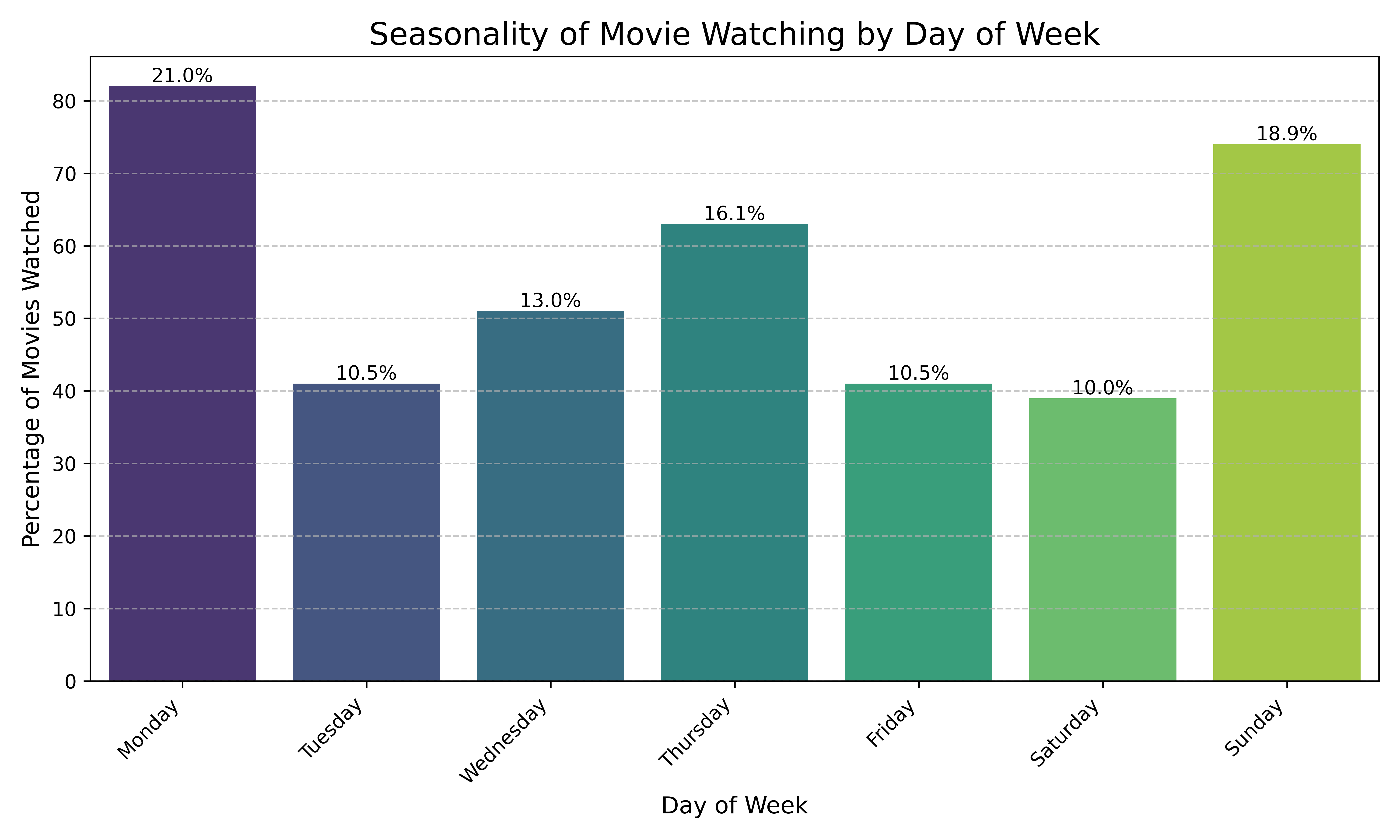
It looks like my preferred day of week to watch movies is… Monday?! 40% of the movies I watched in these years have been watched on Sundays and Mondays. Nice. I did not expect this.
Preferred Genres
Let’s now look at the the distribution of my watched genres.
# Extracting and counting genres for watched movies
genres = watched_movies["Genre"].str.split(", ", expand=True).stack().value_counts()

# Plotting a bar chart of most watched genres
plt.figure(figsize=(10, 6))
sns.barplot(x=genres.index, y=genres.values, palette="viridis")
plt.xticks(rotation=45, ha="right")
plt.xlabel("Genre")
plt.ylabel("Number of Films Watched")
plt.title("Most Watched Genres")
plt.tight_layout()
plt.show()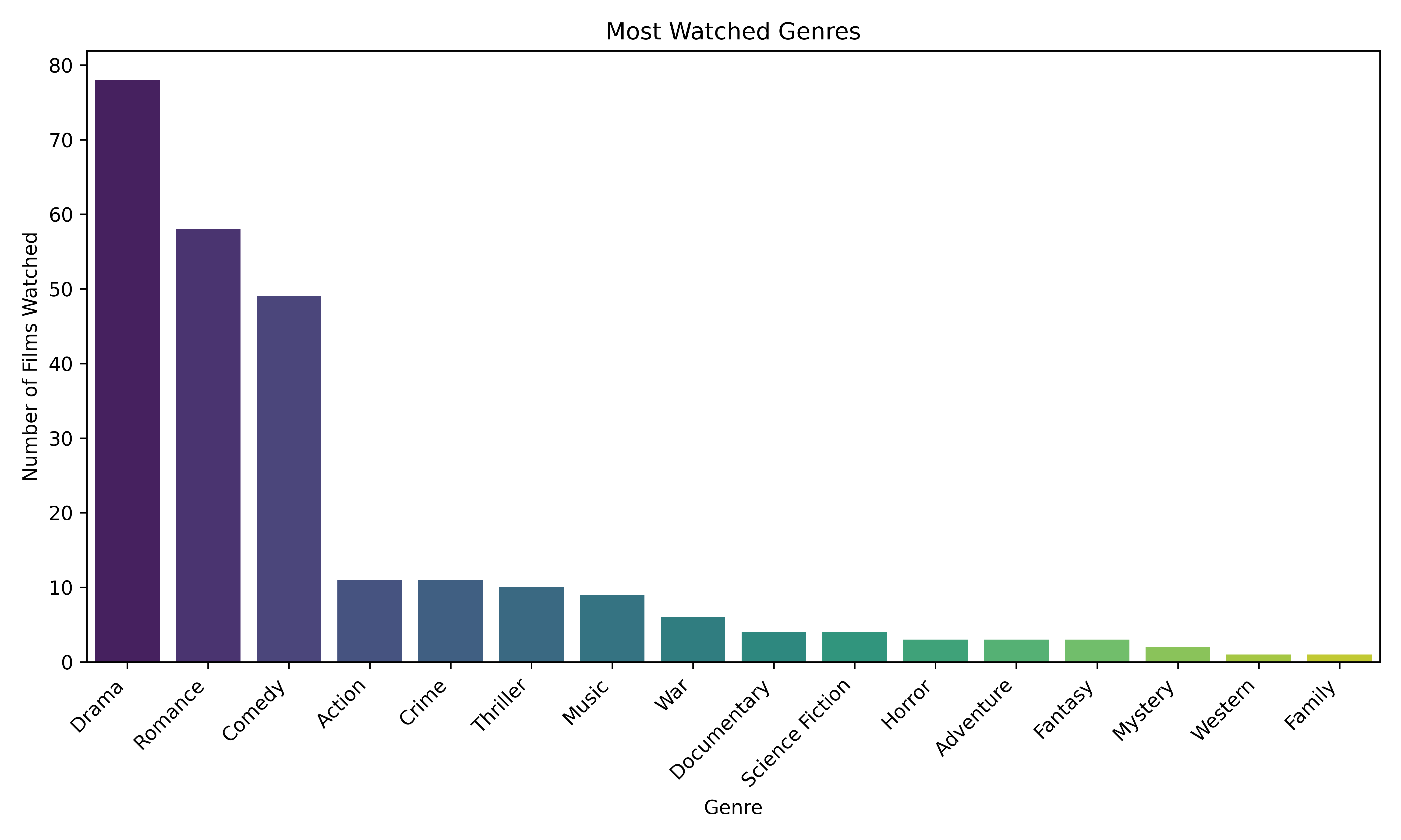
Favourite genre is drama for a drama queen.
Movie Ratings
Let’s visualize the distribution of my ratings.
# Plot a histogram of film ratings for rated movies
rated_movies = watched_movies.dropna(subset=["Rating"])
plt.figure(figsize=(8, 6))
bin_edges = [i / 2 for i in range(2, 21)]
sns.histplot(rated_movies["Rating"], bins=bin_edges, kde=True)
plt.xticks(bin_edges, fontsize=10)
plt.xlabel("Rating")
plt.ylabel("Frequency")
plt.title("Distribution of Film Ratings (Rated Movies)")
plt.show()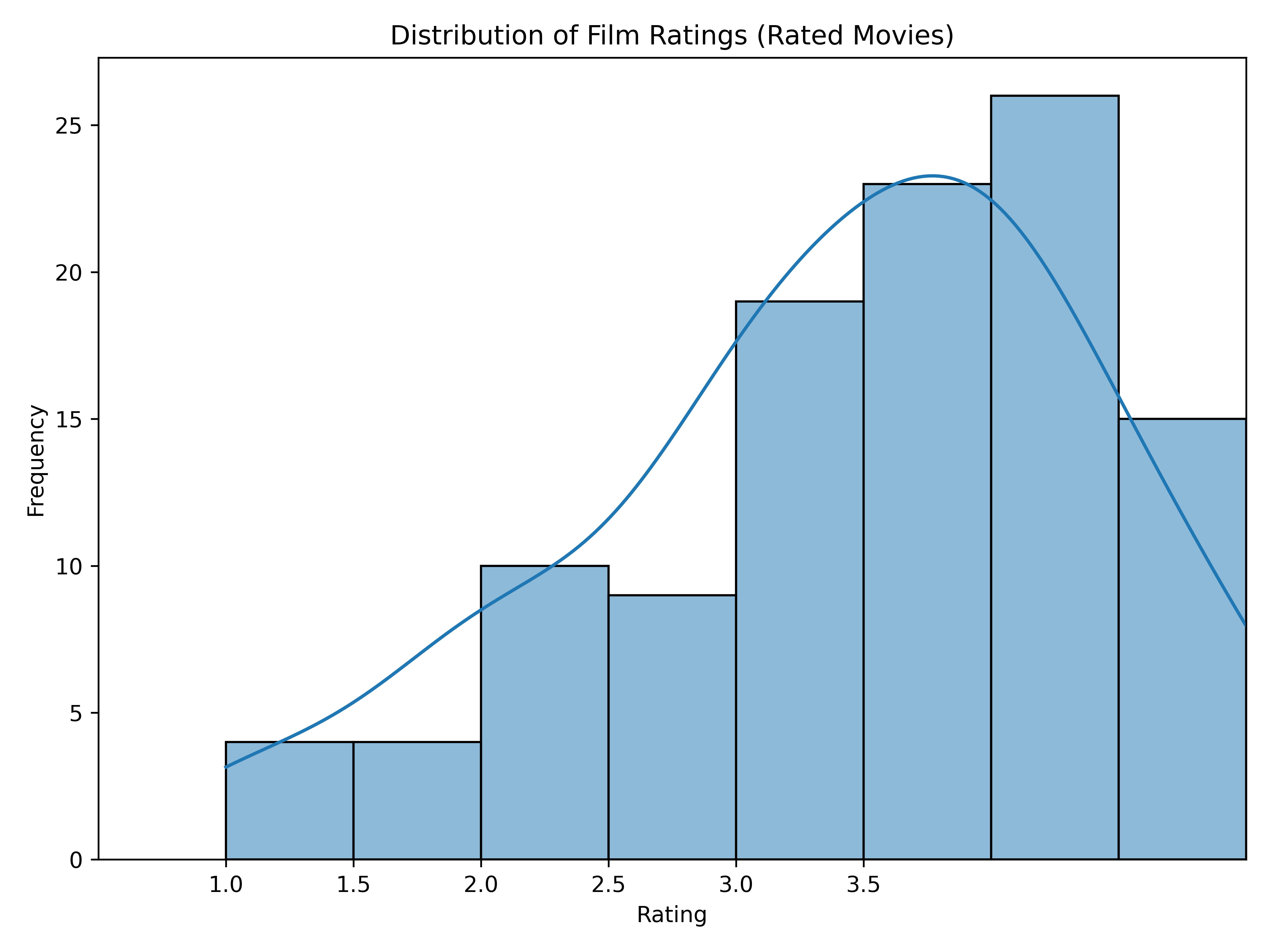
I never gave a 0.5, such a gentle spectator I am!
Average Rating and Film Count by Release Year
I’ll now calculate the number of films watched for each release year, and then I’ll plot both my average rating and the film count.
# Group the rated movies by their release year and calculate the average rating and count of films watched for each year
average_ratings_by_year = rated_movies.groupby("Year")["Rating"].mean()
film_count_by_year = rated_movies["Year"].value_counts()

# Create a figure with two subplots sharing the x-axis
fig, ax1 = plt.subplots(figsize=(10, 6))

# Plot the average ratings on the first subplot (left y-axis)
ax1.plot(average_ratings_by_year.index, average_ratings_by_year.values, marker='o', color='b', label='Average Rating')
ax1.set_xlabel("Release Year")
ax1.set_ylabel("Average Rating")
ax1.set_title("Average Rating and Film Count by Release Year")

# Plot the film count on the second subplot (right y-axis)
ax2 = ax1.twinx()  # Create a second y-axis that shares the same x-axis
ax2.bar(film_count_by_year.index, film_count_by_year.values, alpha=0.5, color='r', label='Film Count')
ax2.set_ylabel("Film Count")

# Show gridlines for both subplots
ax1.grid(True)
ax2.grid(False)

# Combine legends from both subplots
lines, labels = ax1.get_legend_handles_labels()
lines2, labels2 = ax2.get_legend_handles_labels()
ax2.legend(lines + lines2, labels + labels2, loc='upper left')

# Show the plot
plt.show()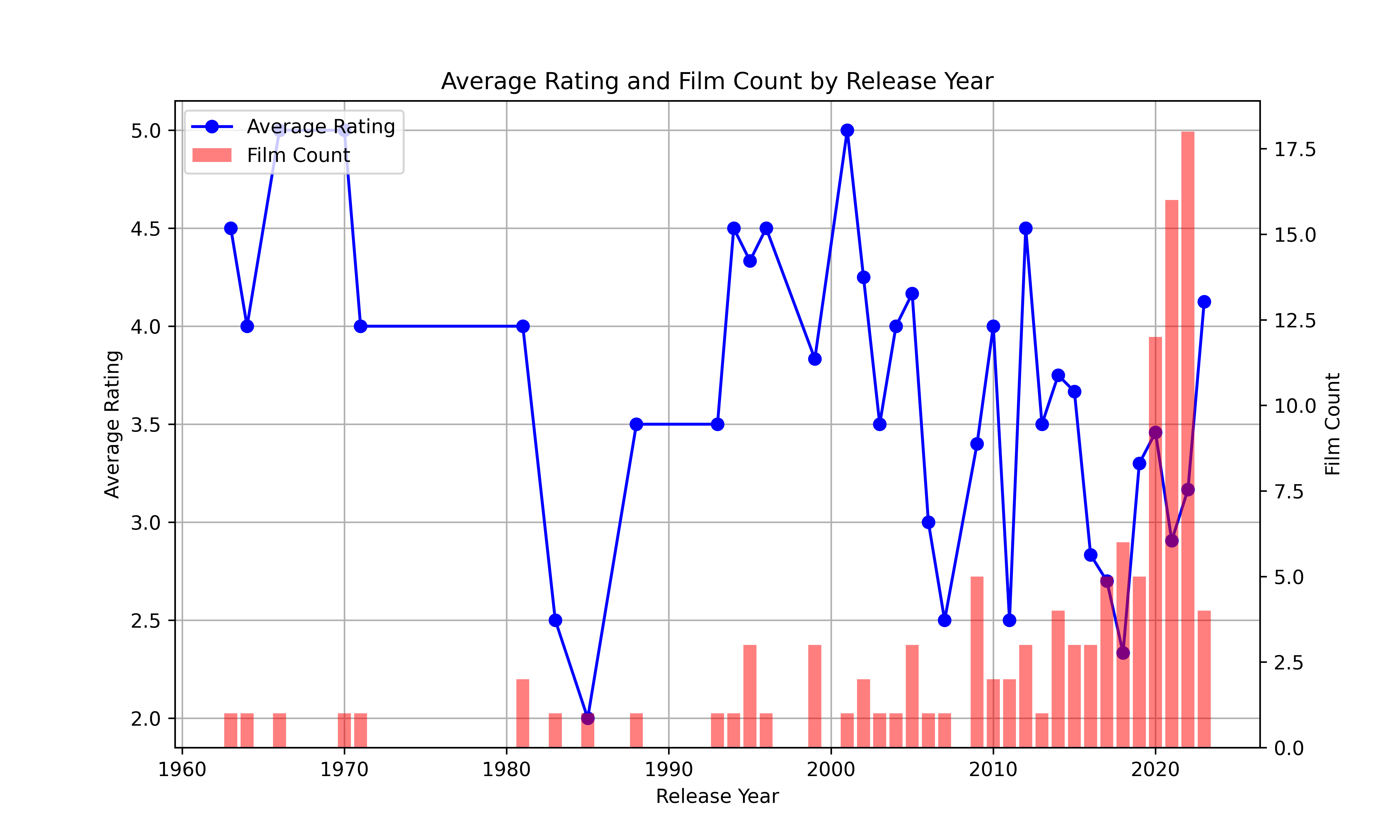
I should definitely fill the gap of movies released in the 70s.
Conclusion
This analysis offered a unique perspective into my movie-watching preferences, highlighting preferred genres, and the presence of a particular day dominance in my movie-watching routine. By leveraging data-driven insights, I can make more informed decisions when selecting movies and continue to enrich my cinematic experience. Too bad that no dataset can (yet) tell me how many times I fell asleep before being able to finish the movies I logged!